You run an A/B test on two deep link destinations. After three days, Variant B has a 6.1% conversion rate versus Variant A's 5.4%. Your frequentist test says "not significant" because you haven't hit the required sample size yet. But you need to make a decision by Friday.
This is where Bayesian A/B testing changes the game. Instead of a binary "significant or not" answer, it tells you: "There is an 87% probability that Variant B is better, and the expected upside is 0.6 percentage points." That's a statement you can actually act on.
For foundational A/B testing concepts, see A/B Testing Deep Links and Landing Pages. For the frequentist approach, see Statistical Significance for A/B Tests.
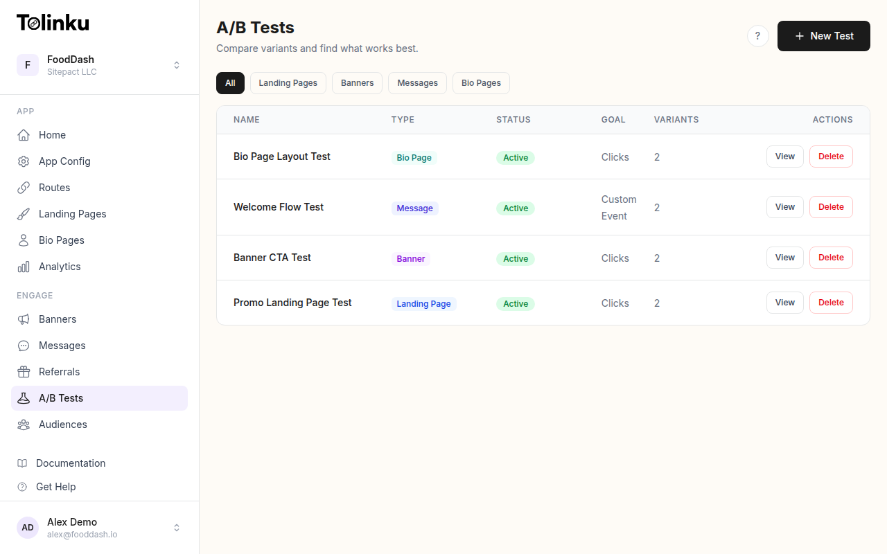 The A/B tests list page showing test names, status, types, and variant counts.
Bayesian vs. Frequentist: The Core Difference
Frequentist A/B testing asks: "If there were no real difference, how likely is this data?" It produces a p-value, which is the probability of seeing your results (or more extreme results) under the assumption that both variants are identical. If that probability is below a threshold (usually 5%), you reject the null hypothesis.
Bayesian A/B testing asks a more direct question: "Given the data I've observed, what's the probability that Variant B is better than Variant A?" It produces a posterior distribution for each variant's true conversion rate, then compares them.
The practical differences matter:
| Frequentist | Bayesian | |
|---|---|---|
| Output | p-value, confidence interval | Probability of being best, credible interval |
| Interpretation | "Reject or fail to reject the null" | "82% chance B is better" |
| Sample size | Must be fixed in advance | Can check results anytime |
| Early stopping | Inflates false positive rate | Built-in; posterior updates continuously |
| Prior knowledge | Not incorporated | Can encode prior beliefs |
For mobile deep link experiments, the Bayesian approach has a significant practical advantage: mobile traffic is often limited, campaigns are short-lived, and you need answers fast. Bayesian methods let you make informed decisions with less data.
The Beta-Binomial Model
For conversion rate experiments (did the user convert or not?), the Beta-Binomial model is the standard Bayesian approach. It works because conversions are binary outcomes, and the Beta distribution is a natural fit for modeling probabilities.
How It Works
Start with a prior. Before seeing any data, you express your belief about the conversion rate using a Beta distribution. A common uninformative prior is Beta(1, 1), which says "any conversion rate between 0% and 100% is equally likely."
Observe data. You collect conversions (successes) and non-conversions (failures) for each variant.
Compute the posterior. The posterior distribution is also a Beta distribution (this is what makes the model elegant). If your prior is Beta(alpha, beta) and you observe
ssuccesses andffailures, the posterior is Beta(alpha + s, beta + f).For example, if Variant A gets 54 conversions out of 1,000 visitors:
- Prior: Beta(1, 1)
- Posterior: Beta(1 + 54, 1 + 946) = Beta(55, 947)
- The posterior mean is 55 / (55 + 947) = 5.49%
The posterior captures your full uncertainty about the true conversion rate. It's not a single number; it's a distribution showing which values are plausible and how plausible each one is.
Computing Key Metrics
Once you have posterior distributions for each variant, you can compute everything you need to make a decision.
Probability of Being Best
This is the headline metric: "What's the probability that Variant B has a higher true conversion rate than Variant A?" You compute it by sampling from both posteriors and counting how often B beats A.
function probabilityBIsBest(alphaA, betaA, alphaB, betaB, samples = 100000) {
  let bWins = 0;

  for (let i = 0; i < samples; i++) {
    const sampleA = betaSample(alphaA, betaA);
    const sampleB = betaSample(alphaB, betaB);
    if (sampleB > sampleA) bWins++;
  }

  return bWins / samples;
}

// Beta distribution sampling using the Joehnk method
function betaSample(alpha, beta) {
  const gammaA = gammaSample(alpha);
  const gammaB = gammaSample(beta);
  return gammaA / (gammaA + gammaB);
}

function gammaSample(shape) {
  // Marsaglia and Tsang's method
  if (shape < 1) {
    return gammaSample(shape + 1) * Math.pow(Math.random(), 1 / shape);
  }
  const d = shape - 1 / 3;
  const c = 1 / Math.sqrt(9 * d);
  while (true) {
    let x, v;
    do {
      x = randn();
      v = 1 + c * x;
    } while (v <= 0);
    v = v * v * v;
    const u = Math.random();
    if (u < 1 - 0.0331 * (x * x) * (x * x)) return d * v;
    if (Math.log(u) < 0.5 * x * x + d * (1 - v + Math.log(v))) return d * v;
  }
}

function randn() {
  const u1 = Math.random();
  const u2 = Math.random();
  return Math.sqrt(-2 * Math.log(u1)) * Math.cos(2 * Math.PI * u2);
}
With 1,000 visitors per variant and conversion rates of 5.4% vs. 6.1%, this might return 0.82, meaning there's an 82% probability that Variant B is genuinely better.
Expected Loss
Probability of being best alone isn't enough. You also want to know: "If I pick B and I'm wrong, how much do I lose?" This is the expected loss (also called risk).
function expectedLoss(alphaA, betaA, alphaB, betaB, samples = 100000) {
  let lossA = 0;
  let lossB = 0;

  for (let i = 0; i < samples; i++) {
    const sampleA = betaSample(alphaA, betaA);
    const sampleB = betaSample(alphaB, betaB);

    // Loss of choosing A when B might be better
    lossA += Math.max(0, sampleB - sampleA);
    // Loss of choosing B when A might be better
    lossB += Math.max(0, sampleA - sampleB);
  }

  return {
    lossIfChooseA: lossA / samples,
    lossIfChooseB: lossB / samples,
  };
}
Expected loss gives you a risk threshold. You might decide: "I'll declare a winner when the expected loss of choosing them is below 0.1 percentage points." This is a more nuanced stopping rule than "wait for p < 0.05."
Credible Intervals
Bayesian credible intervals are the intuitive analog of confidence intervals, but they mean what you probably thought confidence intervals meant all along.
A 95% credible interval for a conversion rate means: "There is a 95% probability that the true conversion rate falls within this range." (A 95% confidence interval does not mean this, despite common misconception. It means that 95% of such intervals, constructed from repeated experiments, would contain the true value.)
function credibleInterval(alpha, beta, level = 0.95) {
  const lower = (1 - level) / 2;
  const upper = 1 - lower;

  return {
    lower: betaQuantile(alpha, beta, lower),
    median: betaQuantile(alpha, beta, 0.5),
    upper: betaQuantile(alpha, beta, upper),
  };
}
For a variant with Beta(55, 947) posterior, the 95% credible interval might be [4.2%, 7.0%]. You can say with 95% probability that the true conversion rate is between 4.2% and 7.0%.
Choosing a Prior
The prior encodes what you know before the experiment starts. For most deep link experiments, you have three reasonable options:
Uninformative prior: Beta(1, 1). This is the uniform distribution. It says you have no prior knowledge. Use this when you're testing something genuinely new and have no baseline data.
Weakly informative prior: Beta(2, 38). This encodes a belief that the conversion rate is "probably around 5%" without being too confident. It's equivalent to having seen 2 conversions out of 40 visitors in a hypothetical previous experiment. Use this when you have a rough sense of your baseline but want the data to dominate quickly.
Empirical prior. If you've run similar experiments before, use that data. If your deep link routes typically convert at 4-7%, you could set a prior like Beta(10, 170), which centers around 5.6% with moderate confidence. The data will still override the prior as observations accumulate.
In practice, the prior matters less than you might think. With even a few hundred observations per variant, the posterior is almost entirely determined by the data. Priors only matter in very small samples.
When to Use Bayesian vs. Frequentist
Bayesian A/B testing is not universally better. Each approach has its strengths.
Use Bayesian when:
- Your traffic is limited (fewer than 5,000 visitors per variant)
- You need to make decisions quickly, before reaching a traditional sample size
- You want intuitive probability statements for stakeholders ("78% chance B is better")
- You're running continuous experiments and checking results regularly
- You want to incorporate prior knowledge from previous experiments
Use frequentist when:
- You have high traffic and can afford to wait for fixed sample sizes
- Regulatory or organizational standards require p-values and confidence intervals
- You need results that are straightforward to audit and reproduce
- You're running a one-off test with a clear stopping point
For mobile deep link experiments on Tolinku, Bayesian methods are often the better fit. Campaign windows are finite, mobile traffic splits across platforms and devices, and product teams want actionable answers, not abstract statistical statements.
A Complete Bayesian Test Workflow
Here's how a Bayesian A/B test flows for a deep link experiment:
Define the experiment. You're testing two deep link destinations: Variant A sends users to the app home screen; Variant B sends them to a personalized recommendations page.
Set the prior. Based on previous campaigns, you know your baseline conversion rate is around 5%. You set Beta(5, 95) as the prior for both variants.
Run the experiment. Traffic splits 50/50. After three days, Variant A has 48 conversions from 900 visitors. Variant B has 63 conversions from 920 visitors.
Compute posteriors.
- Variant A: Beta(5 + 48, 95 + 852) = Beta(53, 947). Mean: 5.3%
- Variant B: Beta(5 + 63, 95 + 857) = Beta(68, 952). Mean: 6.7%
Evaluate.
- Probability B is best: 91.2%
- Expected loss of choosing B: 0.04 percentage points
- Expected loss of choosing A: 1.1 percentage points
- 95% credible interval for lift: [0.1%, 2.7%]
Decide. With a 91% probability that B is better and an expected loss below your threshold (say, 0.1 pp), you can confidently deploy Variant B.
The key advantage here is that you didn't need to wait for a predetermined sample size. You evaluated the evidence as it came in, and the math accounted for the uncertainty at every step.
Best Practices
Set a loss threshold, not a probability threshold. "Probability of being best > 95%" sounds rigorous, but it ignores magnitude. A variant that's 0.01% better will eventually reach 95% probability with enough data. Expected loss (e.g., "less than 0.1 pp") ensures you only act when the decision actually matters.
Run tests for at least one full business cycle. Even with Bayesian methods, day-of-week effects can skew results. Running for at least seven days ensures your posterior reflects the full pattern of user behavior.
Don't ignore practical significance. A 92% probability that Variant B is better sounds compelling. But if the expected improvement is 0.05 percentage points, it might not be worth the engineering effort to deploy. Always pair statistical evidence with business impact.
Use the same prior for all variants. If you give one variant a more optimistic prior, you're biasing the comparison. Start every variant from the same prior and let the data differentiate them.
Document your priors and thresholds. Before starting the test, write down your prior choice, your loss threshold, and your decision criteria. This prevents post-hoc rationalization and keeps your experimentation process honest.
For more on running effective experiments, see A/B Testing Deep Links and Landing Pages and the Tolinku A/B testing documentation.
Get deep linking tips in your inbox
One email per week. No spam.